Jose's Blog

$
\newcommand\R{\mathbb{R}}
$
The last time I think I was serious with Mathematica was 2001? or maybe a few years earlier. I really cannot remember. But I left it and always looked at Maple for enlightenment (where I was/am not still good at). In the past when I looked at Mathematica I thought of it as a Maple similar and probably any amateur would still believe this to be. Both very clumsy to work with. Now, 2016, they differ so much and have advanced so much. One is good at one thing, the other at another. But this is not a debate which is better. This is a “tutorial” what you can do a little good with one. Today Mathematica won my heart (another day it could be Maple). Because the topic “Cylindrical Algebraic Decomposition” (which we in the real world, i.e. real algebraic geometry world, just simply call “cylindrical decomposition”) expresses the strength of Mathematica.

A Mathematica code is a bit different from a C++ code (or even Maple) that I am more used to. So let me list down some things I (think I) learned during the coarse of a few days looking at one or two codes:

• f @ something means apply f to x
• f /@ {a,b,c} means {f[a],f[b],f[c]}
• f @@ List[...] means change List to f
• f @@@ List[List[...]] means List[f[...]]

The first problem that I had is the following: Given an real algebraic set defined by a polynomial function $f:\R^m\rightarrow \R$ , find the number of connected component of the complement of this set. Also find an “algorithm” that can tell if two elements in $\R^m$ belong in the same connected component.

For the sake of argument I took $m=2$ and variables to be $x$ and $y$. Then I wanted to find the connected components of all those $(x,y)$ for which $f(x,y)\neq 0$. To this I copied and modified a code from a mathematica stackexchange post and the modified code looks like this

Coco[eqns_, xrange_: {x, -1, 1}, yrange_: {y, -1, 1}, 
  plotit_: False] := 
 Module[{decomp, connected, regconn}, 
  regconn = 
   Resolve@Exists[{x, y}, (x | y) \[Element] Reals, 
      RegionMember[
       RegionIntersection[ImplicitRegion[#1, {x, y}], 
        RegionBoundary@ImplicitRegion[#2, {x, y}]], {x, y}]] &;
  decomp = 
   List @@ BooleanMinimize@CylindricalDecomposition[eqns, {x, y}];
  connected = 
   Or @@@ ConnectedComponents@
     Graph[decomp, 
      UndirectedEdge @@@ 
       Select[Subsets[decomp, {2}], 
        regconn @@ # || regconn @@ Reverse@# &]];
  Print["number of connected components: ", Length@connected];
  If[plotit,Print[
    (Quiet@
         RegionPlot[#, xrange, yrange, 
          PlotPoints -> 100] & /@ {decomp, connected})~
     Join~{FullSimplify[connected, (x | y) \[Element] Reals]}]]; 
  Return[connected]]

As you can see the code just simplifies the regions defined by cylindrical algebraic decomposition using disjunctive normal form and then finds the regions of intersection by identifying each region as a vertex of a graph and then connecting the vertices if they have common intersections. Then Mathematicas (quit powerful) graph theory package can figure out the connected components of the graph and thus identify exactly the connected components of the Zariski open set defined by the complement of the hypersurface. This, I think, is an overkill. You really need not convert everything into a graph and use Mathematica’s connected component procedure for graph. You just need to use pigeon-hole principal by placing each region in a set containers and iteratively by order fill the set containers depending on common intersection of region or make a new container if there is no existing set container having region with common intersection. Since I was/am a lazy animal and the procedure was fast enough for my purpose, I left it as it was.

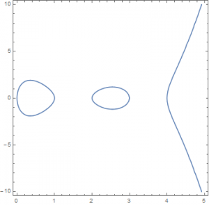
I tested this on a curve for which I knew how many connected components it’s complement have, namely the curve $y^2=x(x-1)(x-2)(x-3)(x-4)$ the plotof which looks like this:

After applying the Coco on the curve by typing (the three other parameters in Coco are optional, they are only used to plot the regions)

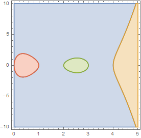
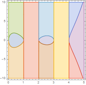
connected = Coco[y^2 != x(x-1)(x-2)(x-3)(x-4),{x,0,5},{y,-10,10},True];

I get the picture for the cylindrical algebraic decompositions

the picture of the different components

the number of components and the actual regions given (click to see in full glory)

The counting of component for this function, without plotting, took around 6.7 seconds in my not-so-fast laptop. Understandably, most of the time was sucked by the plotting. The plotting does not concern me a lot so I am happy with this. I think it can even be made faster (I predict, with correct coding and optimization you can squeeze it to 2 seconds).

Hopefully, in a future post I will show how this is done (with less pictures) when the hypersurface lies in a space with dimension greater than two (i.e. $m>2$).